Canopy Basemap from Lidar
I'm always looking for a way to create a better basemap for my cartographic work. One of my favorite tools is the bare Earth model created by stripping canopy data from LiDAR. Sometimes having tree canopy data is useful for cartographic purposes, so here's a quick tutorial on how I've extracted and symbolized that data for use in ArcMap.
Our goal is to end up with a map that looks like this. I have used a hillshade generated from LiDAR and have it set to 50% transparent and the canopy layer is underneath with a color ramp of leaf green for high, apple green for medium, and yucca yellow for low (none). I've added elevation contours, and a water layer created using this tutorial.

To get to this map, you'll need to have two elevation layers rendered from LiDAR. I'm working with data that can be found here. Feel free to download White_2015_16_zLAS.zip and work alongside me. Once you've got all of your zLAS files in a LAS Dataset, add it to the table of contents and zoom in to view an area. You'll also want to turn on the LAS Dataset from the toolbars menu.
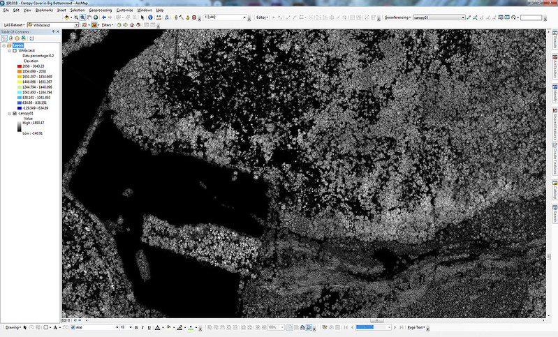
Once the LAS Dataset toolbar is open, make sure the drop down menu Filters is set to All, and the drop down menu with colored dots is set to Elevation, as shown below.


It should render out an image that looks like this hot mess. The "static" looking area is what tree canopy looks like when it's made into a TIN (Triangulated irregular network).

Using the LAS Dataset to Raster tool we'll convert what we see above into a raster image to work with. Let's call it elev_w_canopy since it's a combination of elevation and canopy.

Now let's create a bare Earth model (BEM) where we use the LAS Dataset tools to strip away the canopy.

The resulting terrain should look smoother than the terrain with canopy. Let's use the LAS Dataset to Raster tool to make this into a raster also. Let's call it elev.

Once you've created elev, you can create all kinds of wonderful derivative products from it like contours, and hillshade. Since we're making a map in this tutorial go ahead an render out some contours at 100' intervals, and generate a hillshade for use later.
Now for the magic. Since we have a raster of elev and elev_w_canopy, and what we're after is literally the difference between them, we can use the Raster Calculator tool to execute that.

You'll end up with a raster image that looks something like this. Note that if you zoom in, there will be lots of gaps and the image itself appears noisy and grainy.
Let's deal with that noise by using Focal Statistics. Set the neighborhood to circle, the radius to 8 pixels, and the statistics type to maximum as shown below. Let's call the output canopy01.

You should end up with a raster that looks something like this.

Apply a thoughful color ramp to it, and stretch the histogram appropriately (equalize gets rid of the outliers nicely).

Add your hillshade above the canopy layer now and set your transparency to 50%. You should be looking at something that looks like this.

Our goal is to end up with a map that looks like this. I have used a hillshade generated from LiDAR and have it set to 50% transparent and the canopy layer is underneath with a color ramp of leaf green for high, apple green for medium, and yucca yellow for low (none). I've added elevation contours, and a water layer created using this tutorial.
To get to this map, you'll need to have two elevation layers rendered from LiDAR. I'm working with data that can be found here. Feel free to download White_2015_16_zLAS.zip and work alongside me. Once you've got all of your zLAS files in a LAS Dataset, add it to the table of contents and zoom in to view an area. You'll also want to turn on the LAS Dataset from the toolbars menu.
Once the LAS Dataset toolbar is open, make sure the drop down menu Filters is set to All, and the drop down menu with colored dots is set to Elevation, as shown below.
It should render out an image that looks like this hot mess. The "static" looking area is what tree canopy looks like when it's made into a TIN (Triangulated irregular network).
Using the LAS Dataset to Raster tool we'll convert what we see above into a raster image to work with. Let's call it elev_w_canopy since it's a combination of elevation and canopy.
Now let's create a bare Earth model (BEM) where we use the LAS Dataset tools to strip away the canopy.
The resulting terrain should look smoother than the terrain with canopy. Let's use the LAS Dataset to Raster tool to make this into a raster also. Let's call it elev.
Once you've created elev, you can create all kinds of wonderful derivative products from it like contours, and hillshade. Since we're making a map in this tutorial go ahead an render out some contours at 100' intervals, and generate a hillshade for use later.
Now for the magic. Since we have a raster of elev and elev_w_canopy, and what we're after is literally the difference between them, we can use the Raster Calculator tool to execute that.
You'll end up with a raster image that looks something like this. Note that if you zoom in, there will be lots of gaps and the image itself appears noisy and grainy.
Let's deal with that noise by using Focal Statistics. Set the neighborhood to circle, the radius to 8 pixels, and the statistics type to maximum as shown below. Let's call the output canopy01.
You should end up with a raster that looks something like this.
Apply a thoughful color ramp to it, and stretch the histogram appropriately (equalize gets rid of the outliers nicely).
Add your hillshade above the canopy layer now and set your transparency to 50%. You should be looking at something that looks like this.


Comments